Fortran and Python
P. de Buyl (U of T & Brussels)
SNUG June 2011
Fortran and Python
Background
- Working in physics: statistical mechanics & nonlinear dynamics, mainly.
- Lots of numerical work.
- Mostly Fortran and Python.
Opposite Languages
Python
- An interpreted dynamically typed programming language.
- Quite recent (started in the late 80's)
Fortran
- A strongly typed compiled programming language.
- Quite old (early 50's)
Common points
Python
- NumPy provides a powerful array syntax.
- There are now plenty of scientific libraries. Some of them being wrappers around Fortran libraries.
Fortran
- A powerful array syntax built into the standard.
- A very large body of numerical libraries.
Tools
- Python with NumPy and iPython
http://www.scipy.org/ - A Fortran compiler (the gcc based gfortran works, some commercial compilers also work).
http://gcc.gnu.org/fortran/ - All that is presented today runs on SciNet!
How to use iPython - I
cenoli57:~ pierre$ ssh scinet
scinet03-$ ssh -Y gpc02
gpc-f102n084-$ module load gcc python
gpc-f102n084-$ ipython -pylab
Python 2.6.2 (r262:71600, Oct  9 2009, 11:31:24)
Type "copyright", "credits" or "license" for more information.

IPython 0.10 -- An enhanced Interactive Python.
?         -> Introduction and overview of IPython's features.
%quickref -> Quick reference.
help      -> Python's own help system.
object?   -> Details about 'object'. ?object also works, ?? prints more.

  Welcome to pylab, a matplotlib-based Python environment.
  For more information, type 'help(pylab)'.

In [1]:
How to use iPython - II
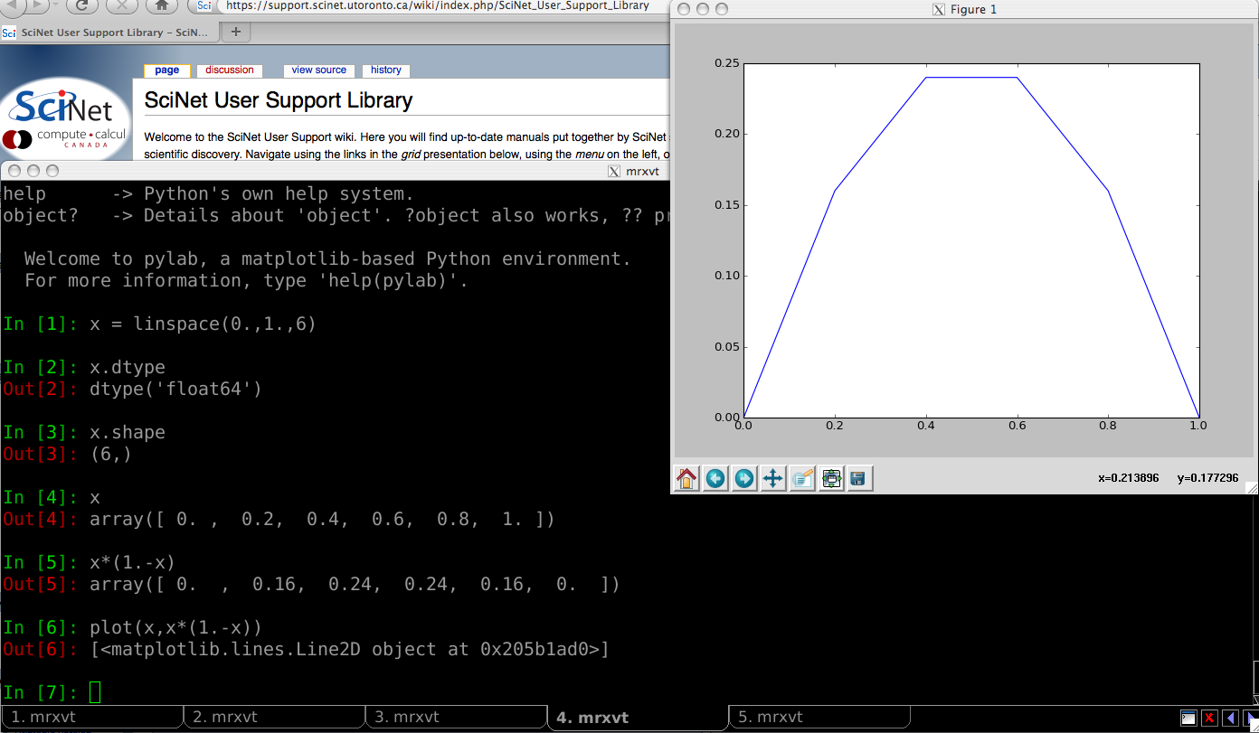
In [21]: x = linspace(0.,1.,6)

In [22]: x.dtype
Out[22]: dtype('float64')

In [23]: x.shape
Out[23]: (6,)

In [24]: x
Out[24]: array([ 0. ,  0.2,  0.4,  0.6,  0.8,  1. ])

In [25]: x*(1.-x)
Out[25]: array([ 0.  ,  0.16,  0.24,  0.24,  0.16,  0.  ])
How to use iPython - III
Introductory example
subroutine multiply(a,b,n,c)
  double precision, intent(in) :: a(n), b(n)
  integer, intent(in) :: n
  double precision, intent(out) :: c(n)
  integer :: i
  do i=1,n
     c(i)=a(i)*b(i)
  end do
end subroutine multiply
import numpy as np ; import my_f90mod
a = np.arange(10,dtype=np.float64) ; a /= len(a)
b = a.copy() ; b /= len(b) ; b = -b + 1.
c = my_f90mod.multiply(a,b)
print(a) ; print(b) ; print(c)
Introductory example - Compiling
gpc-f102n084-$ module load gcc python
gpc-f102n084-$ ls
my_f90mod.f90
gpc-f102n084-$ f2py -m my_f90mod -c my_f90mod.f90
gpc-f102n084-$ ls
my_f90mod.f90  my_f90mod.so
Introductory example - Running
In [1]: import numpy as np ; import my_f90mod

In [2]: a = np.arange(10,dtype=np.float64) ; a /= len(a)

In [3]: b = a.copy() ; b /= len(b) ; b = -b + 1.

In [4]: c = my_f90mod.multiply(a,b)

In [5]: print(a) ; print(b) ; print(c)
[ 0.   0.1  0.2  0.3  0.4  0.5  0.6  0.7  0.8  0.9]
[ 1.    0.99  0.98  0.97  0.96  0.95  0.94  0.93  0.92  0.91]
[ 0.     0.099  0.196  0.291  0.384  0.475  0.564  0.651  0.736  0.819]
A few remarks
- The intent of Fortran arguments is always specified (else, it falls back on the default: intent(in)).
- intent(out) arguments are returned by the Python function.
- "Automatic" information, such as the size of the array, is made optional in the wrapping process.
- This example is useless, from the performance point of view:
- Each calls requires a memory allocation.
- NumPy uses so-called
ufunc's, function that operate on the array at once, calling optimized code.
Array passing
Intent arguments
- intent(in) data is not copied, just a descriptor. It cannot be modified.
- intent(out) a new array is allocated and return by the f2py wrapper.
- intent(inout) the array is made available, can be modified and should already be allocated.
Beware of unwanted copies
- In the following cases, a copy happens anyway.
- Convert the data type.
- The array is non "Fortran".
- The array is non contiguous.
Example
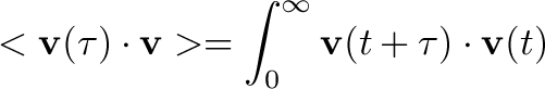
Computation
The computation of the velocity autocorrelation function is really slow in Python.
Speed test
Some results for the speed test.
Computation of 3000 values based on a 90000 elements long dataset.
- NumPy 3.87 seconds
- F2PY 0.76 seconds
Beyond 1D arrays : Array order
Array order
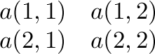
is stored as
 in Fortran
![\( a[1,1]\ a[1,2]\ a[2,1]\ a[2,2] \)](ltxpng/scinet-f2py_d46f977702ac603fddf2fe7b1d0d3c634a450331.png) in C/C++/Python
in C/C++/Python
Problems
The array order problem needs to be taken into account:
- For performance purposes as it impacts memory access performance.
- When doing cross language programming.
Fortran and C orders
C
In [2]: a= np.arange(4);\
        a.shape = (2,2)

In [3]: a
Out[3]:
array([[0, 1],
       [2, 3]])

In [4]: a.flags
Out[4]:
  C_CONTIGUOUS : True
  F_CONTIGUOUS : False
  OWNDATA : True
  WRITEABLE : True
  ALIGNED : True
  UPDATEIFCOPY : False
Fortran
In [5]: b = a.T

In [6]: b
Out[6]:
array([[0, 2],
       [1, 3]])

In [7]: b.flags
Out[7]:
  C_CONTIGUOUS : False
  F_CONTIGUOUS : True
  OWNDATA : False
  WRITEABLE : True
  ALIGNED : True
  UPDATEIFCOPY : False
A personal solution
- To handle the array order, here is a solution
- Work from NumPy as usual.
- Pass the transposed array (
a.Tinstead ofa) to f2py with intent(inout). - Work from Fortran with reversed indices.
- This is fine for situtation with natural locality, such as particles.
- In NumPy, a
r[N,D]array is declared (N=# of particles, D=#of dimensions). - The array
r.Tis passed to Fortran.
- In NumPy, a
Using modules - I
module map
  double precision :: mu, last
  double precision, allocatable :: x(:)
contains
  subroutine iter(x0,n)
    double precision, intent(in) :: x0
    integer, intent(in) :: n
    integer :: i
    if (allocated(x)) deallocate(x)
    allocate(x(n))
    last = x0
    do i=1,n
       last = mu*last*(1.-last)
       x(i) = last
    end do
  end subroutine iter
end module map
Using modules - II
In [1]: from map import map

In [2]: map.x

In [3]: map.mu
Out[3]: array(0.0)

In [4]: map.x = arange(100, dtype=float64)

In [5]: map.x.flags
Out[5]:
  C_CONTIGUOUS : True
  F_CONTIGUOUS : True
  OWNDATA : False
  WRITEABLE : True
  ALIGNED : True
  UPDATEIFCOPY : False
Using modules - III
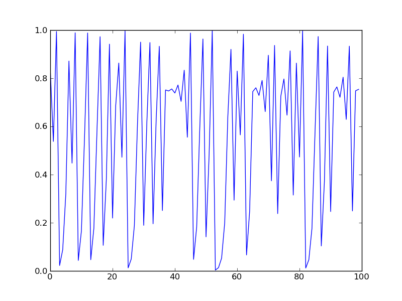
Example
import numpy as np ; import matplotlib.pyplot as plt
from map import map
map.mu = 4.
map.iter(.7, 100)
plt.plot(map.x)
plt.show()
Result
Using modules - IV
Timing the results
import numpy as np
import matplotlib.pyplot as plt
from map import map
from time import clock
mu = 4.
def logistic(x):
    return mu*x*(1.-x)
t1=clock(); data=[]; x=.7
for i in range(10000000):
    x = logistic(x)
    data.append(x)
print "Python ",clock()-t1," s"
t1 = clock()
map.iter(.7,10000000)
print "Fortran ",clock()-t1," s"
Results
- Python 9.87 seconds
- Fortran 0.17 seconds
- For iterative processes (no vectorization), NumPy cannot do miracles.
Beyond this talk
Other methods to speed up Python
- numexpr
- c/c++
- fwrap
Not covered
- f2py allows to specify comment-like directives in Fortran or even a ".pyf" description file.
- Packaging the resulting code
Acknowledgments
![]()
- Prof. R. Kapral
- NSERC Canada
![]()
- Prof. P. Gaspard
- Bureau of International Relations